MatheAss - Stochastics
Statistics
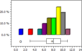
For a master list, the mean (arithmetic mean), the central value (median), the variance and the standard deviation are determined. In addition, the distribution is output as a histogram and as a box plot.
Data:
9 6 7 7 3 9 10 1 8 7 9 6 9 8 10 5 10 10 9 11 8

Number of data        n = 21
Maximum            max = 11
Minimum              min = 1
Mean                        x = 7,7142857
Median                     c = 8
Variance                 s² = 6,1142857
Standard deviation  s = 2,4727082
 Regression
With this routine, you can perform a curve adjustment for a series of measurements. You can choose between the following adjustments and, if necessary, move or stretch all points in the x or y direction.
Proportional regression ( y = a·x )
Linear regression ( y = a·x + b )
Polynomial regression n-th order ( y = a0 + ... + an·xn )
Geometric regression ( y = a·xb )
Exponential regression ( y = a·bx )
Logarithmic regression ( y = a + b·ln(x) )
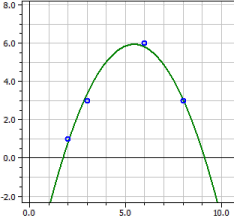
Polynomial Regression

 y =  - 6,9152542
        + 4,7189266·x
        - 0,43361582·x2

Coeff.of determin.   = 0,98338318
Correlation coeff.    = 0,99165679
Standard deviation = 0,46028731
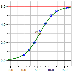
Logistic Regression
(New in version 9.0)
The pogram determines for a series of measurements a curve fit to the logistic function
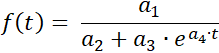
with the parameters a1 = ƒ(0)· S , a2 = ƒ(0) , a3 = S - ƒ(0) ,
and a4 = -k· S and the saturation limit S .
Data from:  "hopfenwachstum.csv"

Saturation limit:  6
      Dark figure:  1

                          4,0189
ƒ(x) = ————————————————
            0,66981 + 5,3302 · e^(-0,35622·t)


Inflection point W(5,8226/3)

Maximum growth rate ƒ'(xw) = 0,53433

8 Values
Coeff.of determin.   = 0,99383916
Correlation coeff.    = 0,99691482
Standard deviation = 0,16172584
Combinatorics
The number of possibilities to select k from n elements is calculated if the order is valued or not and if repetitions are allowed or not.
n = 49
k = 6

Arrangements without repetit. = 10 068 347 520
Arrangements with repetitions = 13 841 287 201
Combinations without repetit. = 13 983 816
Combinations with repetitions = 25 827 165

Permutations of k :        k! = 720
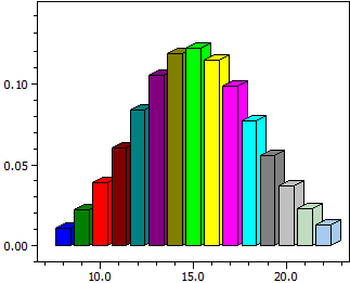
Binomial Distribution
Calculated for a b(k;n;p) distributed random quantity X at fixed n and fixed p
- a rod diagram of the probabilities P(X=k)
- their numerical values in an interval [k-min;k-max]
- the probability P( k-min < = X <= k-max)
n = 50             p = 0,3

    k             P(X=k)         P(0<=X<=k)
  ¯¯¯¯    ¯¯¯¯¯¯¯¯¯¯     ¯¯¯¯¯¯¯¯¯¯
    8         0,01098914     0,01825335
    9         0,02197829     0,04023163
  10        0,03861899     0,07885062
  11        0,06018544     0,13903606
  12        0,08382972     0,22286578
  13        0,10501745     0,32788324
  14        0,11894834     0,44683157
  15        0,12234686     0,56917844
  16        0,11470018     0,68387862
  17        0,09831444     0,78219306
  18        0,07724706     0,85944012
  19        0,05575728     0,91519740
  20        0,03703876     0,95223616
  21        0,02267679     0,97491296
  22        0,01281092     0,98772387
  ¯¯¯¯    ¯¯¯¯¯¯¯¯¯¯     ¯¯¯¯¯¯¯¯¯¯
  P(8<=k<=22)   =          0,98045967
Hypergeometric Distribution
Calculations are made for a random variable X distributed h (k; n; m; r) with a fixed n, m and fixed r a bar chart and a table of values for the probabilities P(X=k).
Normal Distribution
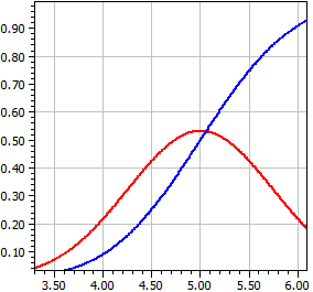
Calculations are carried out for an N(µ, σ2) distributed random variable X with a given expected value µ and variance σ2 , the density function ƒ(x) and the distribution function Φ(x), i.e. the integral over ƒ(x).
  μ = 5 ,      σ = .75

         x                    ƒ(x)                Φ(x)
  ¯¯¯¯¯¯¯¯¯¯  ¯¯¯¯¯¯¯¯¯¯  ¯¯¯¯¯¯¯¯¯¯
  2                    0,00017844   0,00003167
  2,33333333   0,00095649   0,00018859
  2,66666666   0,00420802   0,00093192
  2,99999999   0,01519465   0,00383038
  3,33333332   0,04503153   0,01313415
  3,66666665   0,10953585   0,03772017
  3,99999998   0,21868009   0,09121120
  4,33333331   0,35832381   0,18703139
  4,66666664   0,48189843   0,32836063
  4,99999997   0,53192304   0,49999998
  5,3333333     0,48189845   0,67163934
  5,66666663   0,35832383   0,81296859
  5,99999996   0,21868012   0,90878878
  6,33333329   0,10953586   0,96227982
  6,66666662   0,04503154   0,98686585
  6,99999995   0,01519465   0,99616962
  7,33333328   0,00420802   0,99906808
  7,66666661   0,00095649   0,99981141
  7,99999994   0,00017844   0,99996833